
Systematic Strategy 1: Moving Average Crossover
Systematic Trading Strategy

In a world competing for technological innovation, the role of discretionary vs systematic trading is a large topic for debate. While both play a role in the correct contexts, we present the first of our systematic strategies. The aim is to show both sides of trading, and we introduce systemised trading through a simple moving average crossover strategy1. Simple is the key word, as we will build on the strategies with levels of complexity, stricter risk management levels and more interesting targets to meet.
For now, the target was to create a (somewhat) successful strategy which may be deployed to a live system. We will present a breakdown of what the strategy is, how it is tested, the results of the test and how we can use it across multiple assets.
What is a systematic trading strategy?
Before we begin with the strategy itself, we must describe what a systematic strategy is:
Systematic strategies use pre-defined rules and conditions to make trading decisions (long/short). Implemented based on an algorithm ensures strategies follow the rules for the entire duration the strategy is running and eliminates emotion and bias from the process which may arise in discretionary trading.
Systematic trading focuses on the quantitative processes underlying the algorithms to deliver a consistent strategy. Intense testing and optimisation allow for these strategies to be tailored towards specific markets or products, and install discipline in the trading process.
What is our Moving Average Crossover Strategy?
There are many classes of systematic trading strategies, and our moving average crossover strategy falls under the trend-following category.
This group of strategies believe there are persistent trends in global markets over time, and models can be created to profit from the momentum of these trends.
Our strategy is a variation of this, utilising Exponential Moving Averages (EMA) as its foundation. These moving average assign greater weight to more recent data points and respond to price changes faster than simple moving averages (SMA). Depending on the time-frame of the EMA, we can analyse different characteristics:
Short EMA (10,20): used to analyse short-term trends as sensitive to recent price movements
Long EMA (50,100,200): used to analyse longer-term trends
We use the 20-short-EMA and the 50-long-EMA and define our crossover event as when the two EMA overlap each other.
Long Condition: EMA20 > EMA50 (short EMA crosses above long EMA)
Short Condition: EMA20 < EMA50 (short EMA crosses below long EMA)
In general, in an uptrend, prices tend to move higher over time, reaching higher highs and higher lows. The short-EMA will be more responsive, and adjust to upward price movement faster. This means the short-EMA will be above the slow-moving long-EMA.
Conversely, in a downtrend, prices move lower over time, reaching lower highs and lower lows. By the same logic, the short-EMA will be below the slow-moving long-EMA.
This is the fundamental strategy we are testing today; it is a simple one to start with. More complexities and technical indicators can be added to accompany this one, but sticking with one can isolate the effects of the EMA.
Implementing our strategy
Now we have defined the conditions for entry, however with a systematic strategy there are some further metrics we must tell our algorithm.
For a beginner strategy, we have set a fixed contract size of 1000 shares for each trade initiated. In later strategies we demonstrate how we can create dynamic position sizes depending on equal equity allocation or weighted shares.
An interesting addition we have made to the strategy is to add a lag between successive trades. We want to wait 10 bar lengths (depends on individual bar timeframe) before entering a new position, so that we are not buying and selling too much if there is multiple crossover of the EMAs in a short space of time. This will help bring down transaction costs in a live setting.
We have set a trailing stop-loss to manage the risk of our trades. This is set at 2%, meaning if the trading price falls below (rises above) 2% of the current close price for the long (short) trade, we automatically exit our position. This is to limit downside risk from trading.
To keep things simple for now, we have set commission costs as 0%. We require margins of 10% for both long and short strategies. In practice, the short-margin is typically larger, and our margin requirements may be larger based on individual brokers.
We are testing the strategy over an 8-year period:
Results
The output of this strategy is essentially a custom indicator. This is used to implement trade signals on any underlying asset we want. This is the versatility of systematic strategies.
We explore this strategy on the SPX index in detail:

We see a snapshot of the overlay of the strategy on the SPX daily chart for end of 2022 and 2023 (so-far). We see signals where there is a crossover of our EMA curves and either the long or short orders on the graph.
Total return: 23.99%
Average historical benchmark (SPX) return: 18%
Sharpe ratio: 0.038
Percent profitable: 43.33%
Average time trades open for: 4 days
Here are just a summary of some of the statistics from our backtests. While we see that overall return has beaten the long-term S&P historical average by 6%, we note some downsides to the model which suggest return is not the only factor to consider.
We have not considered commission costs, which we will include in a later model
On average we have more losing trades than winning trades as winning percent is less than 50%. This means the average winning trade is larger than the average losing trade. While this is good, more losing trades is a concerning sign
Our sharp ratio is positive, but low. This means we are generating risk-adjusted returns above the risk-free rate benchmark, but not significantly higher. We will explore methods to increase this in future strategies
Our trades are on average open for 4 days. Winning trades are open for an average of 7 days. Losing trades are open for an average of 2 days. It may be worth modifying models in the future to allow for further lags before sending successive orders to allow trades to run their course before they are exited without hitting target profit levels
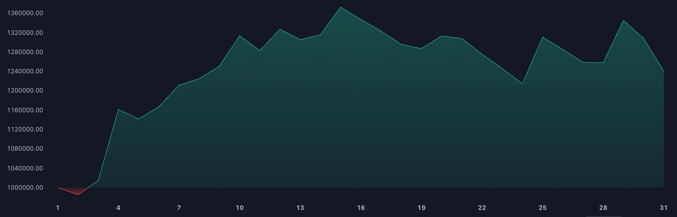
Below we see the equity curve for this strategy, which shows equity holdings over the testing range of the strategy (8 years). We generally look for smooth equity curves as they indicate more consistent performance over time.
Further thoughts
We have considered the daily timeframe and the SPX for this strategy. We may be able to test this against different timeframes and see whether the strategy works better on some than others. Also, we can test it on different products other than the SPX, as the versatility of this strategy means it can be applied to any asset.
GOLD - XAUUSD
We test the same strategy against the gold pair XAUUSD (gold/US$). We switch the timeframe of our bar data from daily to 3-hour bars.

The results display a 17.22% return for XAUUSD in the period 13 January, 2021 - 20 July 2023. We have to use a shorter timeframe due to the frequency of the data being higher, and so we adjust accordingly.
If we were to simply buy and hold Gold in the same time period as we traded, our return would be 6.28%. Our Sharpe ratio is higher at 0.237, and our profitable percent has seen a slight improvement at 48.19%.
Our strategy represents a 10.94% improvement on a passively managed investment
Indeed, we proceed with caution as this is again without commission fees. However, we can still see how one strategy which works for the SPX under certain circumstances can work under a different asset in different circumstances. This is the power of systematic trading.
We have seen a simple strategy, which under (very very) simplified assumptions has beaten a passive buy and hold strategy. We look to explore more systematic strategies, building on our trend-following one but deepening our insights into other classes. We can adjust the parameters, arguments, conditions and timeframes to achieve different results depending on our views and assumptions.
Systematic trading is a unique space where innovation is not only encouraged but required to develop efficient algorithms. Managing the levels of risk and reward is a tricky balancing act, but with the right practice; achievable.
If you would like the source code, please subscribe and reply to that email for the code.