
Systematic Strategy 2: Fibonacci Breakout
Systematic Strategy for SPY and NIFTY

Today we preview the second of our systematic strategies, aimed at providing a foundational understanding of passive investing and an unconventional branch of trading. We understood the nuances of what a systematic strategy is and consists of in a previous post, which you can have a look at on this link below:
Systematic Strategy 1: Moving Average Crossover

In a world competing for technological innovation, the role of discretionary vs systematic trading is a large topic for debate. While both play a role in the correct contexts, we present the first of our systematic strategies.
In this, we looked at a simple Moving Average crossover strategy, aimed at capturing momentum swings, which would be reflected through a 20-EMA and 50-EMA overlap. We categorised this as a trend-following strategy, and today we look at another strategy of this class.
Fibonacci Retracement Levels
As explained in the previous article, a trend-following strategy believes there is a particular price movement which it believes will persist for the near future.
You may have come across Fibonacci in a Maths lesson, learning about the sequence of numbers formed by adding the previous 2 together. In the context of trading, we use Fibonacci Retracement levels, which are derived from this sequence:
Retracement levels are calculated as follows:
21/21 = 100%
21/34 = 61.8%
21/55 = 38.2%
21/89 = 23.6%
Although 50% is not technically a Fibonacci Retracement level, we often include it in a trading concept because it provides a useful level as we will see. We can continue this pattern and retrieve more granular levels, however using these retracement levels are the most common:
0%, 23.6%, 38.3%, 50%, 61.8%, 100%
So what is the purpose of these numbers? They are useful in technical analysis for defining our support and resistance levels:
Support levels - price levels at which a down-trending asset tends to halt its movement and find a price floor. There is concentration of demand pressure leading to the pause in downtrend. If buying pressure is large, may be a reversal upward, but there may be a continuation below the support price.
Resistance levels - price levels at which a up-trending asset tends to halt its movement and find a price ceiling. There is concentration of selling pressure leading to the pause in uptrend. If selling pressure is large, may be a reversal downward, but there may be a continuation above the resistance price.
These are not clearly marked labels on a price graph, nor are they the same for each asset at each time. But what Fibonacci Retracement levels allow us to do, is narrow down the search to potential levels. The specific price levels, as % between two chosen prices, may be potential support or resistance levels, depending on the current trend.

It is more of a psychological level than anything. If so many traders are aware of the Fibonacci levels, and that they may be a turning point for price, if price approaches these levels, traders will look to enact buy or sell signals due to a pre-conditioned mindset. It is also the reason we use 50% as a level; because as a midpoint it is a psychological indicator for people. It is not a hard-and-fast rule that prices must halt at the Fib levels, but since so many traders expect it will, it very often translates into reality. The expectation itself leads to a self-fulfilling outcome.
Fibonacci Breakout Strategy
Turning our attention now to our strategy and how we can use the Fibonacci tools to our advantage. When price reaches a Fib level, there are one of 2 possible outcomes:
Prices continue in the trend they were before hitting the level
Prices reverse the trend
Our strategy focuses on the first. We believe in the momentum of the asset.
To determine our points of entry, we rely on the Fib levels. We can therefore generate both BUY signals and SELL signals:
A BUY signal is generated when price breaks through the resistance level to continue the uptrend. More specifically, a BUY signal is generated when the last closing price is above the highest resistance level.
A SELL signal is generated when price breaks through the support level to continue the downtrend. More specifically, a SELL signal is generated when the last closing price is below the lowest support level.
These both define prices where we have broken the support/resistance levels and do not expect a reversal anymore. To solidify the signals, we also impose another rule: both BUY and SELL signals are only sent if the short-term moving average of volume is greater than the long-term moving average of volume.
This ensures there is enough liquidity to continue the uptrend. If we see a fall in volume, it indicates unwillingness to buy or sell, and so we should not expect significant price movements, hence this rule ensures we can continue the trend.
Strategy Parameters
Already we can see our strategy is more advanced than our first. We are not only calculating support and resistance levels, but implementing them along with a volume rule. The aggregation of multiple indicators usually provides a more assured reason to buy or sell, rather than just one. However, using too many indicators may be too restrictive or potentially overfitting the model.
To describe exhaustively the components of the strategy we initialise several parameters as follows:
Daily Lookback = 30
Number of past days’ data to use when calculating Fibonacci Retracement levels
Frequency = 5mins
This is how often we call on data to update our Fib levels and any new trading signals
Stop Loss = 7.5%
Margin = 20%
Short SMA = 20
Used to calculate short-term moving average of volume
Long SMA = 50
Used to calculate long-term moving average of volume
The strategy operates with these parameters. Before market open, it calculates whether there is sufficient capital. Before market close, it squares off all our positions, so we do not have any pending trades or open trades at the end of the day. Currently we have commission costs and slippage costs set to 0 for simplicity.
Results: SPY
First, we test the strategy against the SPY index.
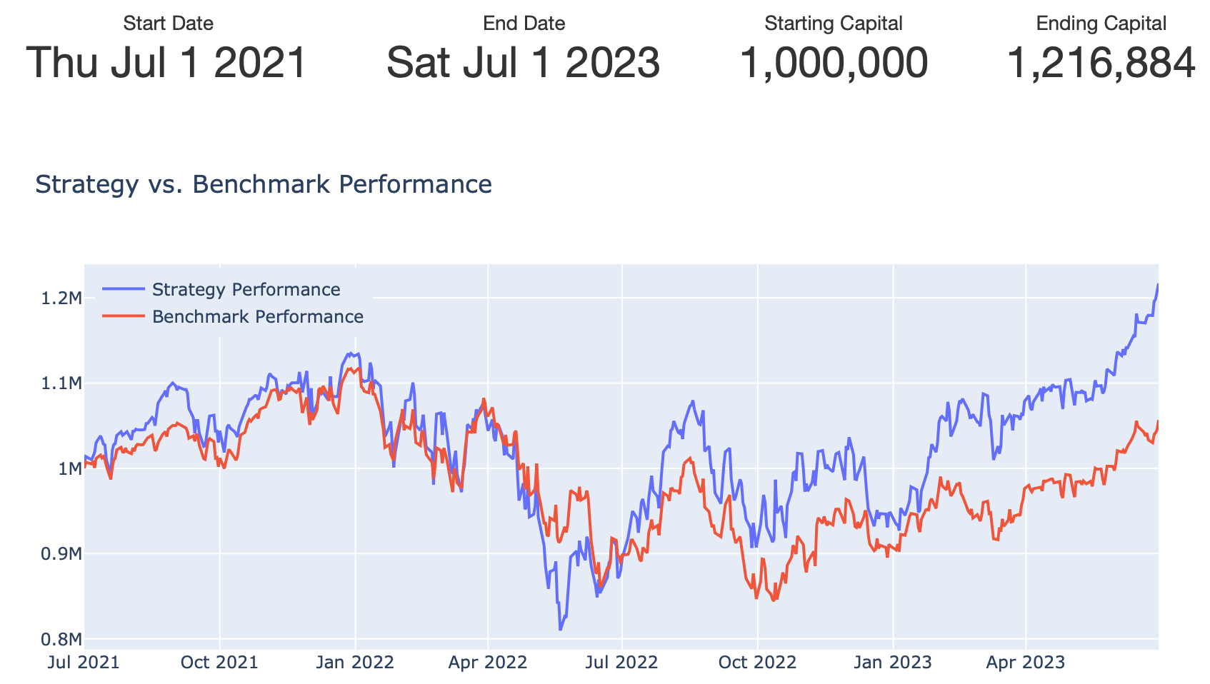
Over a 2-year backtest, we notice that our strategy returned 21.7% relative to the SPY return of 5.7%. A volatile period means that our annual volatility was high around 25%, and this is also reflected in a Sharpe ratio of 0.51. Although returns were strong, there is still downside risk as seen around May/June 2022. This is partly reflective of wider market conditions, and we do see the breakout strategy performing well towards 2023, in spite of some SPY lagged performance.
This strategy did manage to generate an alpha of 0.08. This represents the excess return above a benchmark. A strategy can still generate a positive return but have a negative alpha, if it did not beat the benchmark, however a positive alpha (although small) indicates the breakout strategy did succeed over this timeframe.
There are many simplifications made within the strategy that boost but also hinder performance, such as 0 commission, 0 slippage, 20% margin, fixed lot size of 4000, fixed stop-loss of 7.5%.
Some adjustments may be made to the stop-loss to add a trailing element and also a dynamic position sizing element to enhance performance, however this will be balanced out somewhat by the introduction of commission and slippage costs. Implementing these will be the goal of future strategies, as we improve the precision and reproducibility to a live trading environment.
However, for now the aim is to introduce different styles of strategy which may work or not on various markets, and try to generate some alpha and return, which this strategy was able to do.
But after building a strategy, we want to see whether it can be used in different contexts. For after all, a mistake would be to build a strategy for a particular situation. This is what overfitting is. To modify a strategy and fine-tune it to work for a specific asset for a specific period of time may well have generated returns, but it is not efficient in the sense we cannot employ it across markets. Building a model and strategy based on an idea, fundamental or technical, which can then be fine-tuned based on specific market characteristics (such as lot-sizes or liquidity differences) is a stronger approach.
But, building a strategy fit for multiple markets is easier said than done.
Results: NIFTY/BANKNIFTY
NIFTY is the NSE’s equivalent of the SPY. It tracks the top 50 most liquid companies on the Indian exchange, and BANKNIFTY, as you may have guessed, represents the top 12 most liquid banking stocks in India.
For demonstration purposes, we test the same strategy with the same parameters on these indices, with a modified lot-size, accounting for price differentials. We also test it for the same period, to keep everything consistent.

Now, we notice a few things:
Overall, the strategy returned 22.6%, which although is higher in absolute terms than the SPY strategy, it ended closer to the NIFTY benchmark, on which a buy-and-hold strategy would have returned 22.2%. This suggests that the performance relative to the benchmark was not as strong.
Sharpe ratio was 0.5. This is similar to the SPY strategy, indicating some consistency.
What is evident in this price graph especially, is the volatility of returns. Compared to the benchmark, our strategy shows higher highs but also lower lows. When NIFTY crashes, our strategy is expected to fall, but the drawdown we see (difference between a local peak and trough) is much larger than the benchmark’s drawdown. In addition, when NIFTY rallies, our strategy outperforms it significantly.
Overall this volatility is reflective in the alpha, and overall we generated a -0.02 alpha, and much higher beta (indicative of volatility) of 1.44 vs 1.05 for SPY. The alpha is interesting and confusing. We beat the benchmark at the end, but still generated a negative alpha. However, this is not uncommon. What this means is there was a spike at the end, in which our strategy performed well to beat the benchmark, but over the period, on average we were on par or slightly below.
This is likely driven by the sharp drops, muting the positive effects of the strategy.
Overall, we see that the strategy did generate positive returns, positive alpha for the SPY and on-par alpha for NIFTY. There are merits with the strategy, and an improvement to the parameterisation may lead to prevention of the large volatility we see, to generate a more stable time-series and consistency in returns.